Geoids Fit to North America

In geodetic applications, a geoid represents an equipotential surface of the Earth’s gravity field that closely corresponds to global mean sea level (MSL). It acts as a reference for orthometric heights, which are used in topographic maps, engineering, and water resource studies.

Unlike global geoid models (e.g., EGM2008 or EGM96), which provide undulations relative to a geocentric ellipsoid (an ellipsoid centered at the Earth’s center of mass), North American regional geoid models are computed in a reference frame aligned with the North American plate. The ellipsoid origin in a plate-fixed frame differs from the geocenter by roughly 2.2 meters, which, if not accounted for, would produce meter-scale offsets in ellipsoidal heights. Regional geoid undulation models incorporate dense regional gravity measurements, GPS-on-benchmark data, and other local observations to define the equipotential surface relative to that plate-fixed ellipsoid. Subsequent refinements, such as new airborne/terrestrial gravity surveys (e.g., GRAV-D), updated geoid–quasigeoid separation methods, and improved interpolation—introduce further decimeter-level or smaller adjustments to the geoid undulation field.

It’s important to note that the geoid is not itself a vertical datum, though it underpins vertical datums: a vertical datum uses a geoid model but adds conventions, benchmarks, and adjustment networks to maintain a consistent height system over time and space.

NOAA’s Geoid Models¶

NOAA’s National Geodetic Survey (NGS) develops and maintains a series of regional geoid models for the U.S. and its territories. These include:

• GEOID03
• GEOID09
• GEOID12B
• GEOID18

Each new model integrates improved data and techniques:

• GEOID03 was the first full release using hybrid modeling with GPS-on-benchmark (GPSBM) constraints.
• GEOID09 added more GPSBM control and updated gravimetric models.
• GEOID12B introduced further refinement, particularly for areas impacted by subsidence and uplift.
• GEOID18 is the most recent geoid (not for long!) and is used for the 2022 update to the National Spatial Reference System, includes dramatically better gravity data (from GRAV-D airborne surveys), new GPSBM data, and enhanced interpolation methods. See the technical details for more information.

Originally, these models were distributed as ASCII raster grids that provided geoid undulation (height above the reference ellipsoid) values. While these ASCII files are still available (e.g. https://geodesy.noaa.gov/PC_PROD/GEOID03/) the data is now also hosted as Cloud-Optimized GeoTIFFs (COGs) on cdn.proj.org. This modern format is much more efficient and accessible for direct use in geospatial software and cloud-based workflows, as it allows for streaming only the required portions of the data. In this notebook, we will read these COG files directly into xarray.DataArray objects to visualize and compare them.

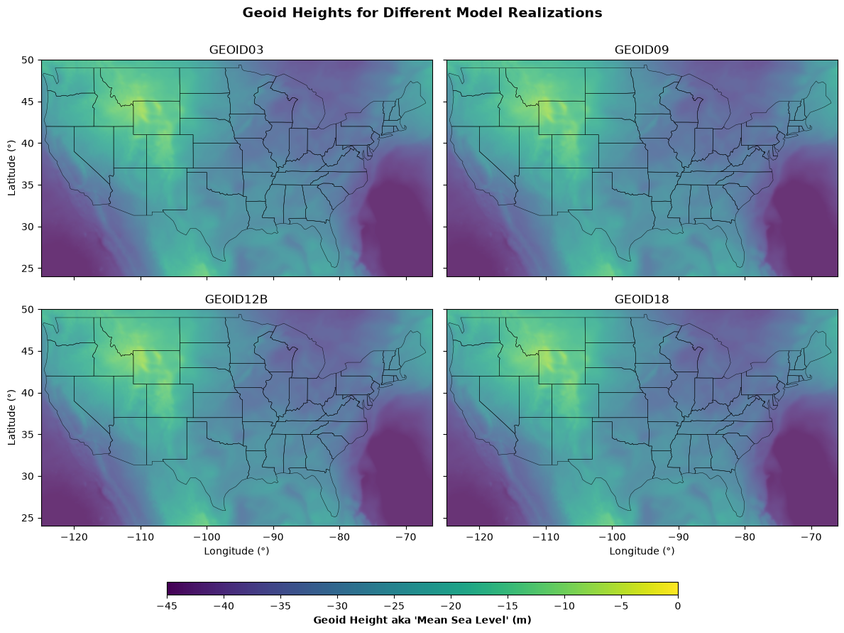
Geoid Heights from Four Model Realizations¶

When visualized directly, the geoid models appear nearly identical to the eye, especially when plotted with a colorbar spanning the full range of mean sea level (-45 to 0 meters across the U.S.). This masks subtle differences between the models that may be critical in applications requiring centimeter-level accuracy.

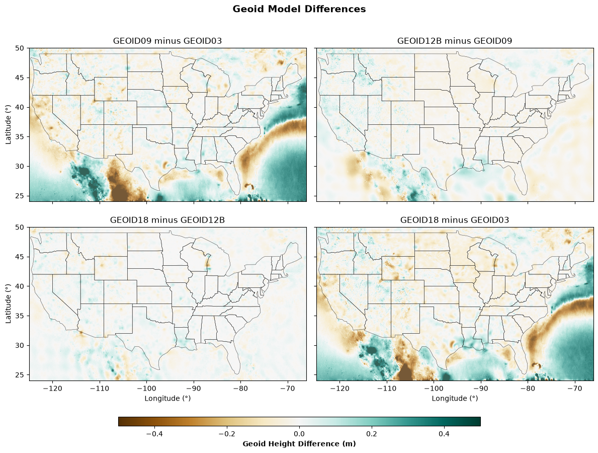
Differences Between Geoid Models¶

The difference plots reveal key insights:

• The GEOID09 - GEOID03 and GEOID18 - GEOID03 comparisons show changes of up to ±0.5 meters, indicating substantial regional updates.
• In contrast, GEOID12B - GEOID09 and GEOID18 - GEOID12B show much smoother and smaller transitions, suggesting evolutionary refinements.

The biggest changes appear:

• Along the Pacific coast, particularly the plate boundary zones in California and the Pacific Northwest. These areas are very tectonically active, and GPSBM data or updated gravity data contributed to significant geoid corrections.
• Across northern Mexico, including Sonora and Chihuahua. Sparse previous coverage combined with new data largely drove greater corrections here.
• Offshore and near the continental margins, where gravity modeling is often more uncertain.
• A notable curving anomaly from Florida up the East Coast and then out into the Atlantic suggests a gravity signal possibly linked to ancient tectonic structures or variations in the continental shelf.
• In southern Ontario and Quebec, glacial isostatic adjustment and post-glacial rebound influence the shape of the geoid.

These patterns highlight how new data acquisition, seismic activity, and better modeling of geophysical processes contribute to iterative geoid improvement.

Why Do These Differences Matter?¶

Even though a 0.5 meter change might seem small, in geodesy and Earth science, these discrepancies can be critical:

• Flood risk mapping: FEMA and other agencies require accurate elevations to model inundation zones. A decimeter error could misclassify properties, and thus flood insurance (which is not cheap).
• Volcanology and deformation monitoring: Height changes on the order of centimeters are relevant when tracking inflation or deflation of magma chambers. Remember Mt. St. Helens in 1980? And the fact that volcanic eruptions can cost airlines millions of dollars per day due to flight disruptions
• Air and sea navigation: Aviation safety and hydrographic charting rely on consistent vertical datums.

Inaccuracies in the geoid can cascade into large errors in derived products. This is why NOAA’s ongoing refinement of the geoid is foundational for geospatial science and infrastructure across North America.